Soft Actor-Critic (SAC)
Overview
The Soft Actor-Critic (SAC) algorithm extends the DDPG algorithm by 1) using a stochastic policy, which in theory can express multi-modal optimal policies. This also enables the use of 2) entropy regularization based on the stochastic policy's entropy. It serves as a built-in, state-dependent exploration heuristic for the agent, instead of relying on non-correlated noise processes as in DDPG, or TD3 Additionally, it incorporates the 3) usage of two Soft Q-network to reduce the overestimation bias issue in Q-network-based methods.
Original papers: The SAC algorithm's initial proposal, and later updates and improvements can be chronologically traced through the following publications:
- Reinforcement Learning with Deep Energy-Based Policies
- Soft Actor-Critic: Off-Policy Maximum Entropy Deep Reinforcement Learning with a Stochastic Actor
- Composable Deep Reinforcement Learning for Robotic Manipulation
- Soft Actor-Critic Algorithms and Applications
Reference resources:
- haarnoja/sac
- openai/spinningup
- pranz24/pytorch-soft-actor-critic
- DLR-RM/stable-baselines3
- denisyarats/pytorch_sac
- haarnoja/softqlearning
- rail-berkeley/softlearning
| Variants Implemented | Description |
|---|---|
sac_continuous_actions.py, docs |
For continuous action space |
Below is our single-file implementations of SAC:
sac_continuous_action.py
The sac_continuous_action.py has the following features:
- For continuous action space.
- Works with the
Boxobservation space of low-level features. - Works with the
Box(continuous) action space. - Numerically stable stochastic policy based on openai/spinningup and pranz24/pytorch-soft-actor-critic implementations.
- Supports automatic entropy coefficient \(\alpha\) tuning, enabled by default.
Usage
poetry install

# Pybullet
poetry install -E pybullet

## Default
python cleanrl/sac_continuous_action.py --env-id HopperBulletEnv-v0

## Without Automatic entropy coef. tuning
python cleanrl/sac_continuous_action.py --env-id HopperBulletEnv-v0 --autotune False --alpha 0.2
Explanation of the logged metrics
Running python cleanrl/ddpg_continuous_action.py will automatically record various metrics such as actor or value losses in Tensorboard. Below is the documentation for these metrics:
-
charts/episodic_return: the episodic return of the game during training -
charts/SPS: number of steps per second -
losses/qf1_loss,losses/qf2_loss: for each Soft Q-value network \(Q_{\theta_i}\), \(i \in \{1,2\}\), this metric holds the mean squared error (MSE) between the soft Q-value estimate \(Q_{\theta_i}(s, a)\) and the entropy regularized Bellman update target estimated as \(r_t + \gamma \, Q_{\theta_{i}^{'}}(s', a') + \alpha \, \mathcal{H} \big[ \pi(a' \vert s') \big]\).
More formally, the Soft Q-value loss for the \(i\)-th network is obtained by:
with the entropy regularized, Soft Bellman update target: $$ y = r(s, a) + \gamma ({\color{orange} \min_{\theta_{1,2}}Q_{\theta_i^{'}}(s',a')} - \alpha \, \text{log} \pi( \cdot \vert s')) $$ where \(a' \sim \pi( \cdot \vert s')\), \(\text{log} \pi( \cdot \vert s')\) approximates the entropy of the policy, and \(\mathcal{D}\) is the replay buffer storing samples of the agent during training.
Here, \(\min_{\theta_{1,2}}Q_{\theta_i^{'}}(s',a')\) takes the minimum Soft Q-value network estimate between the two target Q-value networks \(Q_{\theta_1^{'}}\) and \(Q_{\theta_2^{'}}\) for the next state and action pair, so as to reduce over-estimation bias.
-
losses/qf_loss: averageslosses/qf1_lossandlosses/qf2_lossfor comparison with algorithms using a single Q-value network. -
losses/actor_loss: Given the stochastic nature of the policy in SAC, the actor (or policy) objective is formulated so as to maximize the likelihood of actions \(a \sim \pi( \cdot \vert s)\) that would result in high Q-value estimate \(Q(s, a)\). Additionally, the policy objective encourages the policy to maintain its entropy high enough to help explore, discover, and capture multi-modal optimal policies.
The policy's objective function can thus be defined as:
where the action is sampled using the reparameterization trick1: \(a = \mu_{\phi}(s) + \epsilon \, \sigma_{\phi}(s)\) with \(\epsilon \sim \mathcal{N}(0, 1)\), \(\text{log} \pi_{\phi}( \cdot \vert s')\) approximates the entropy of the policy, and \(\mathcal{D}\) is the replay buffer storing samples of the agent during training.
-
losses/alpha: \(\alpha\) coefficient for entropy regularization of the policy. -
losses/alpha_loss: In the policy's objective defined above, the coefficient of the entropy bonus \(\alpha\) is kept fixed all across the training. As suggested by the authors in Section 5 of the Soft Actor-Critic And Applications paper, the original purpose of augmenting the standard reward with the entropy of the policy is to encourage exploration of not well enough explored states (thus high entropy). Conversely, for states where the policy has already learned a near-optimal policy, it would be preferable to reduce the entropy bonus of the policy, so that it does not become sub-optimal due to the entropy maximization incentive.
Therefore, having a fixed value for \(\alpha\) does not fit this desideratum of matching the entropy bonus with the knowledge of the policy at an arbitrary state during its training.
To mitigate this, the authors proposed a method to dynamically adjust \(\alpha\) as the policy is trained, which is as follows:
where \(\mathcal{H}\) represents the target entropy, the desired lower bound for the expected entropy of the policy over the trajectory distribution induced by the latter. As a heuristic for the target entropy, the authors use the dimension of the action space of the task.
Implementation details
CleanRL's sac_continuous_action.py implementation is based on openai/spinningup.
-
sac_continuous_action.pyuses a numerically stable estimation method for the standard deviation \(\sigma\) of the policy, which squashes it into a range of reasonable values for a standard deviation:Note that unlike openai/spinningup's implementation which usesLOG_STD_MAX = 2 LOG_STD_MIN = -5 class Actor(nn.Module): def __init__(self, env): super(Actor, self).__init__() self.fc1 = nn.Linear(np.array(env.single_observation_space.shape).prod(), 256) self.fc2 = nn.Linear(256, 256) self.fc_mean = nn.Linear(256, np.prod(env.single_action_space.shape)) self.fc_logstd = nn.Linear(256, np.prod(env.single_action_space.shape)) # action rescaling self.action_scale = torch.FloatTensor((env.action_space.high - env.action_space.low) / 2.0) self.action_bias = torch.FloatTensor((env.action_space.high + env.action_space.low) / 2.0) def forward(self, x): x = F.relu(self.fc1(x)) x = F.relu(self.fc2(x)) mean = self.fc_mean(x) log_std = self.fc_logstd(x) log_std = torch.tanh(log_std) log_std = LOG_STD_MIN + 0.5 * (LOG_STD_MAX - LOG_STD_MIN) * (log_std + 1) # From SpinUp / Denis Yarats return mean, log_std def get_action(self, x): mean, log_std = self(x) std = log_std.exp() normal = torch.distributions.Normal(mean, std) x_t = normal.rsample() # for reparameterization trick (mean + std * N(0,1)) y_t = torch.tanh(x_t) action = y_t * self.action_scale + self.action_bias log_prob = normal.log_prob(x_t) # Enforcing Action Bound log_prob -= torch.log(self.action_scale * (1 - y_t.pow(2)) + 1e-6) log_prob = log_prob.sum(1, keepdim=True) mean = torch.tanh(mean) * self.action_scale + self.action_bias return action, log_prob, mean def to(self, device): self.action_scale = self.action_scale.to(device) self.action_bias = self.action_bias.to(device) return super(Actor, self).to(device)LOG_STD_MIN = -20, CleanRL's usesLOG_STD_MIN = -5instead. -
sac_continuous_action.pyuses different learning rates for the policy and the Soft Q-value networks optimization.while openai/spinningup's uses a single learning rate ofparser.add_argument("--policy-lr", type=float, default=3e-4, help="the learning rate of the policy network optimizer") parser.add_argument("--q-lr", type=float, default=1e-3, help="the learning rate of the Q network network optimizer")lr=1e-3for both components.Note that in case it is used, the automatic entropy coefficient \(\alpha\)'s tuning shares the
q-lrlearning rate:# Automatic entropy tuning if args.autotune: target_entropy = -torch.prod(torch.Tensor(envs.single_action_space.shape).to(device)).item() log_alpha = torch.zeros(1, requires_grad=True, device=device) alpha = log_alpha.exp().item() a_optimizer = optim.Adam([log_alpha], lr=args.q_lr) else: alpha = args.alpha -
sac_continuous_action.pyuses--batch-size=256while openai/spinningup's uses--batch-size=100by default.
Experiment results
To run benchmark experiments, see benchmark/sac.sh. Specifically, execute the following command:
The table below compares the results of CleanRL's sac_continuous_action.py with the latest published results by the original authors of the SAC algorithm.
Info
Note that the results table above references the training episodic return for sac_continuous_action.py, the results of Soft Actor-Critic Algorithms and Applications reference evaluation episodic return obtained by running the policy in the deterministic mode.
| Environment | sac_continuous_action.py |
SAC: Algorithms and Applications @ 1M steps |
|---|---|---|
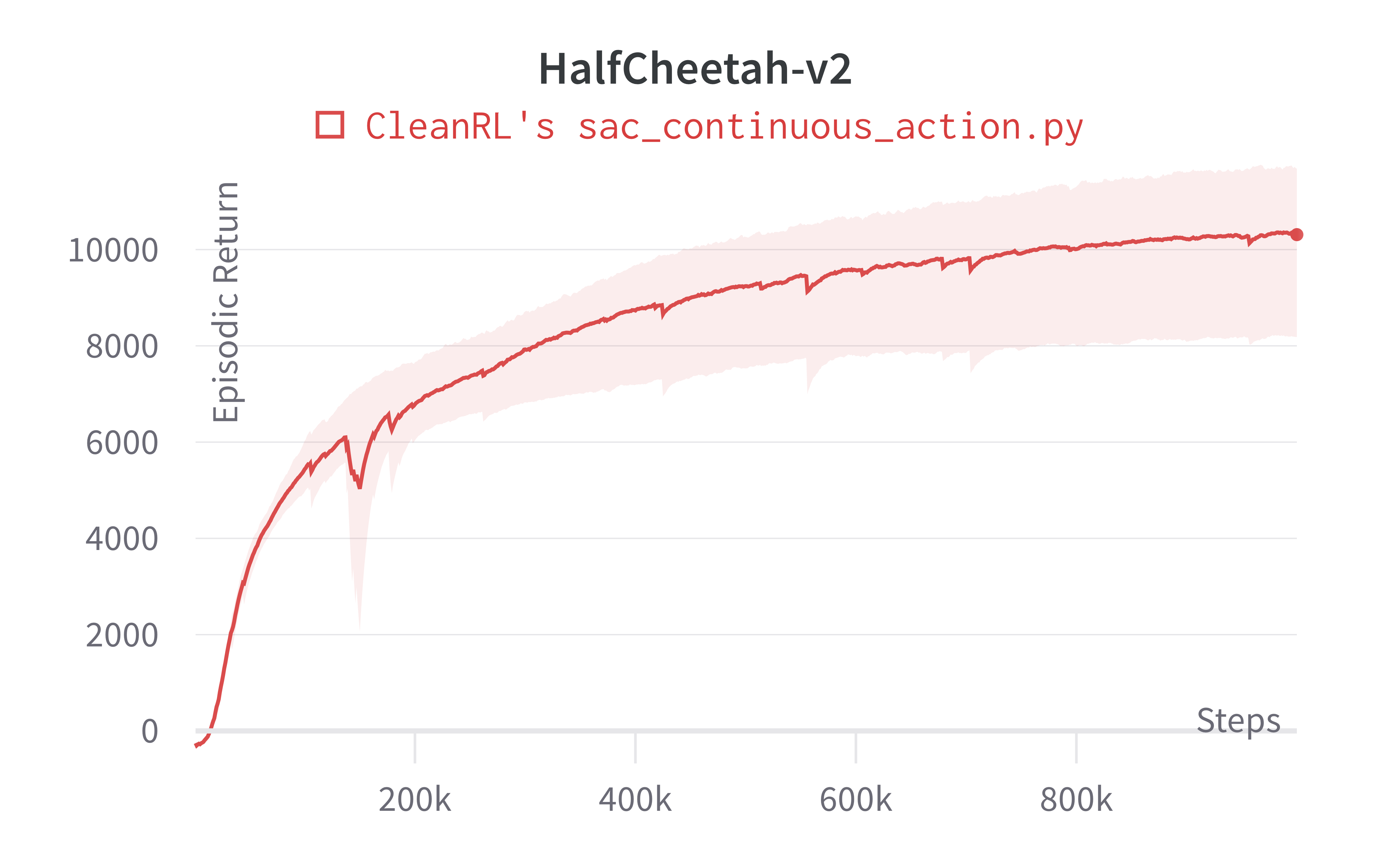
| HalfCheetah-v2 | 10310.37 ± 1873.21 | ~11,250 |
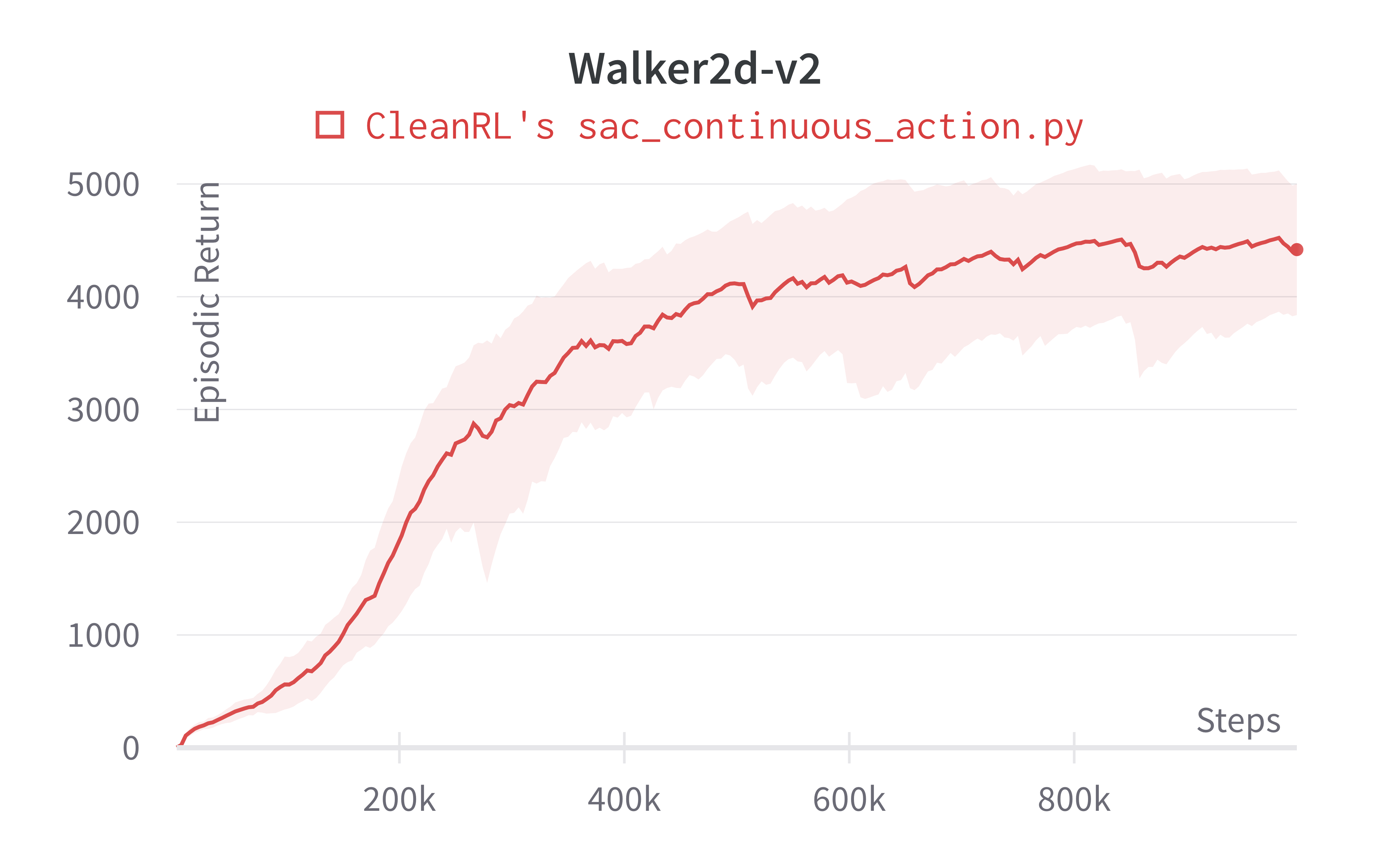
| Walker2d-v2 | 4418.15 ± 592.82 | ~4,800 |
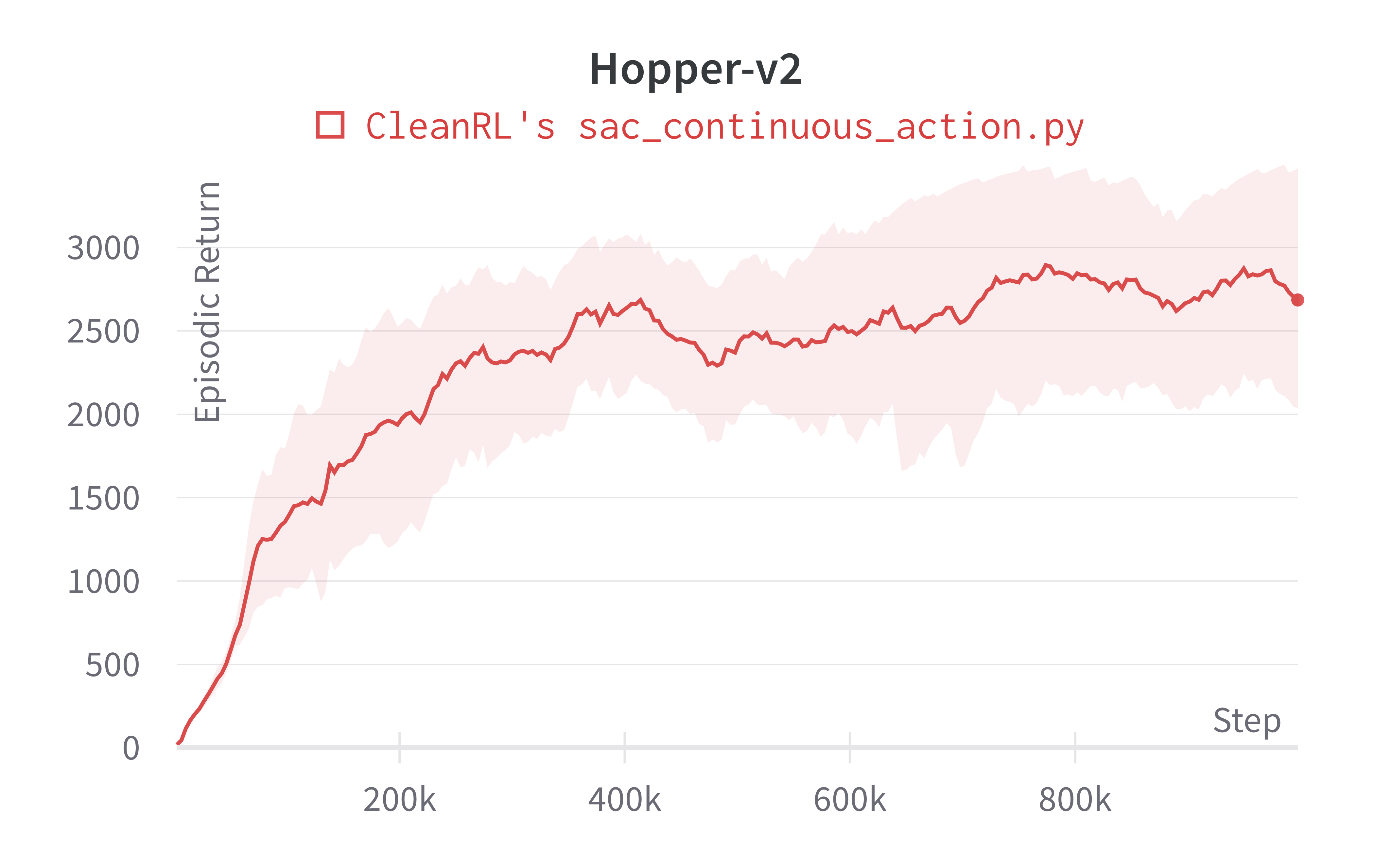
| Hopper-v2 | 2685.76 ± 762.16 | ~3,250 |
Learning curves:
Tracked experiments and game play videos:
-
Diederik P Kingma, Max Welling (2016). Auto-Encoding Variational Bayes. ArXiv, abs/1312.6114. https://arxiv.org/abs/1312.6114 ↩